A Flexible Generalized Linear Mixed Effects Model for Testing Cell-Cell Colocalization in Spatial Immunofluorescent Data
Slide Deck
Overview
This module focuses on testing cell-cell interaction (colocalization)
using spatial regression, implemented in the R package
spaMM.
Load data and libraries.
# required packages
library(tidyverse)
library(spaMM)
theme_set(theme_bw() + theme(legend.position = "bottom"))

# load processed ovarian cancer data
load(url("https://github.com/julia-wrobel/MI_tutorial/raw/main/Data/ovarian.RDA"))
Visualize cell colocalization
We visualize two samples from the ovarian cancer dataset from VectraPolarisData and colocalization of B-cells and CD8- T-cells. We are interested in testing if this colocalization is significant (i.e., more interaction than random chance), and if it correlates with five-year survival.
# create five-year survival variable
ovarian_df <- ovarian_df %>%
  mutate(vysurvival = case_when(
    survival_time >= 60  ~ 1,
    death == 1 ~ 0,
    TRUE ~ NA_real_
  ))

# cell phenotype variable
ovarian_df <- ovarian_df %>%
  mutate(phenotype = case_when(
    phenotype_cd68 == "CD68+" ~ "macrophage",
    phenotype_cd19 == "CD19+" ~ "B-cell",
    phenotype_cd3 == "CD3+" & phenotype_cd8 == "CD8+" ~ "CD8+ T-cell",
    phenotype_cd3 == "CD3+" & phenotype_cd8 == "CD8-" ~ "CD8- T-cell",
    TRUE ~ "other"
  ))

# subset to two samples with moderate B-cell populations
subjs_subset <- ovarian_df %>%
  filter(!is.na(vysurvival)) %>%
  group_by(sample_id, vysurvival) %>%
  filter(any(phenotype == "macrophage"),
         any(phenotype == "B-cell"),
         any(phenotype == "CD8+ T-cell"),
         any(phenotype == "CD8- T-cell")) %>%
  summarise(n_b_cells = sum(phenotype == "B-cell")) %>%
  filter(n_b_cells < 100) %>%
  group_by(vysurvival) %>%
  arrange(-n_b_cells) %>%
  slice(1) %>%
  pull(sample_id)

ovarian_df_subset <- ovarian_df %>%
  filter(sample_id %in% subjs_subset)

# visualize B-cells and CD8- T-cells across images
p_viz <- ovarian_df_subset %>%
  group_by(sample_id) %>%
  mutate(x_viz = x - min(x),
                y_viz = y - min(y)) %>%
  mutate(phenotype_viz = phenotype %>%
                  recode(
                    "CD8+ T-cell" = "other",
                    "macrophage" = "other") %>%
                  factor(levels = c("other", "CD8- T-cell", "B-cell"))) %>%
  arrange(phenotype_viz) %>%
  ggplot(aes(x_viz, y_viz, color = phenotype_viz, size = phenotype_viz)) +
  geom_point(alpha = 0.5) +
  scale_color_manual(values = c("B-cell" = "red",
                                "CD8- T-cell" = "blue",
                                "other" = "grey")) +
  scale_size_manual(values = c("B-cell" = 0.5,
                                "CD8- T-cell" = 0.5,
                                "other" = 0.2)) +
  facet_wrap(~ paste0("vysurvival ", vysurvival) +
               paste0("sample_id ", sample_id), nrow = 1) +
  # annotation for 25 micron scale bar
  annotate(geom = "segment", x = 10, y = 10, xend = 35, yend = 10) +
  annotate(geom = "text", x = 22.5, y = 10, label = "25",
           hjust = 0.5, vjust = -0.5) +
  coord_fixed() +
  theme(legend.position ="bottom",
        axis.text = element_blank(),
        axis.ticks = element_blank(),
        panel.grid = element_blank())
print(p_viz)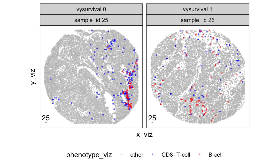
Permutation test for cell colocalization
Here we adopt a permutation based approach to test for cell-cell interaction. This was used in e.g. histoCAT.
Red vertical lines indicate observed number of B-cell/CD8- T-cell interactions in each image.
Histogram indicates number of interactions from randomly permuting cell phenotype labels.
This approach can test for enrichment of interactions in each image, but is difficult to generalize across images, and to test for interaction correlation with phenotypes/outcomes.
threshold <- 25

# construct adjacency matrices for each image
l_mat_adj <- ovarian_df_subset %>%
  group_split(sample_id) %>%
  map(function(i_ovarian_df) {
    mat_dist <- i_ovarian_df %>%
      select(x, y) %>%
      as.matrix() %>%
      dist() %>%
      as.matrix()
    dimnames(mat_dist) <- list(i_ovarian_df$cell_id, i_ovarian_df$cell_id)
    mat_adj <- mat_dist < threshold
    # don't count cell as its own neighbor
    diag(mat_adj) <- 0

    return(mat_adj)
  })

# visualize permuted interaction vs observed interaction
n_perm <- 500
set.seed(0)
df_interactions <- ovarian_df_subset %>%
  group_split(sample_id) %>%
  map2_dfr(l_mat_adj, function(i_ovarian_df, i_mat_adj) {
    n_observe <- sum(i_mat_adj[i_ovarian_df$phenotype == "B-cell",
                                i_ovarian_df$phenotype == "CD8- T-cell"])
    n_permute <- seq(1, n_perm) %>%
      map_dbl(function(i_perm) {
        i_ovarian_df_perm <- i_ovarian_df %>%
          sample_n(size = nrow(.), replace = FALSE)
        sum(i_mat_adj[i_ovarian_df_perm$phenotype == "B-cell",
                       i_ovarian_df_perm$phenotype == "CD8- T-cell"])
      })
    tibble(
      sample_id = i_ovarian_df$sample_id[1],
      vysurvival = i_ovarian_df$vysurvival[1],
      n_observe = n_observe,
      n_permute = n_permute
    )
  })

p_interactions <- df_interactions %>%
  ggplot(aes(x = n_permute)) +
  geom_histogram(bins = 50) +
  geom_text(data = df_interactions %>% filter(!duplicated(sample_id)),
             aes(label = paste0("#interactions from data=", n_observe)),
            x = Inf, y = Inf,
            vjust = 1.2, hjust = 1.05,
            color = "red") +
  geom_vline(data = df_interactions %>%
               filter(sample_id == 26) %>%
               filter(!duplicated(sample_id)),
             aes(xintercept = n_observe), color = "red") +
  facet_wrap(~ paste0("vysurvival ", vysurvival) +
               paste0("sample_id ", sample_id), nrow = 1) +
  xlab("#interactions from permutation")
print(p_interactions)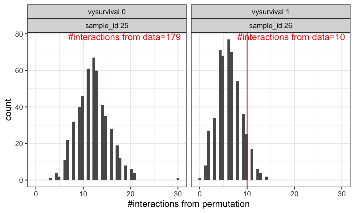
Test for cell colocalization using spatial regression
We can perform spatial regression on each B-cell’s local neighborhood, and the enrichment of CD8 T-cells in each neighborhood.
Visualize the local neighborhood of one B-cell
# calculate number of neighboring cells for each B-cell
df_nb <- ovarian_df_subset %>%
  group_split(sample_id) %>%
  map2_dfr(l_mat_adj, function(i_ovarian_df, i_mat_adj) {
    # count the number of neighbors for each B-cell
    i_df_nb <- i_mat_adj[i_ovarian_df$phenotype == "B-cell", ] %>%
      apply(1, function(x) tapply(x, i_ovarian_df$phenotype, sum)) %>%
      t() %>%
      as.data.frame() %>%
      rownames_to_column("cell_id") %>%
      mutate(total = `B-cell` + `CD8- T-cell` + `CD8+ T-cell` + macrophage + other,
             sample_id = i_ovarian_df$sample_id[1]) %>%
      # remove singletons
      filter(total > 0)

    return(i_df_nb)
  })
df_nb <- df_nb %>%
  mutate(cell_id = as.numeric(cell_id)) %>%
  left_join(ovarian_df_subset,
            by = c("sample_id", "cell_id"))

# visualize the local neighborhood of a particular B-cell
df_one_cell <- df_nb %>%
  filter(sample_id == 25) %>%
  arrange(-`CD8- T-cell`) %>%
  slice(1)
nbs <- l_mat_adj[[1]][as.character(df_one_cell$cell_id), ] %>%
  keep(~.x > 0) %>%
  names() %>%
  as.numeric()
nbs <- c(nbs, df_one_cell$cell_id)
df_cell_viz <- ovarian_df_subset %>%
  filter(sample_id == 25) %>%
  filter(x < df_one_cell$x + 30 & x > df_one_cell$x - 30,
         y < df_one_cell$y + 30 & y > df_one_cell$y - 30)
p_cell_viz <- df_cell_viz %>%
  mutate(phenotype_viz = phenotype %>%
                  recode(
                    "CD8+ T-cell" = "other",
                    "macrophage" = "other") %>%
                  factor(levels = c("other", "CD8- T-cell", "B-cell"))) %>%
  ggplot(aes(x = x, y = y,
             color = phenotype_viz,
             size = cell_id == df_one_cell$cell_id)) +
  geom_point() +
  scale_color_manual(values = c("B-cell" = "red", "CD8- T-cell" = "blue",
                                "other" = "grey")) +
  # don't show size legend
  scale_size_manual(values = c("TRUE" = 3, "FALSE" = 2), guide = "none") +
  # draw a neighborhood circle around the center cell
  annotate("path",
           x = df_one_cell$x + 25*cos(seq(0,2*pi,length.out=100)),
           y = df_one_cell$y + 25*sin(seq(0,2*pi,length.out=100)),
           color = "red",
           linetype = "dashed") +
  coord_fixed() +
  theme(axis.ticks = element_blank(),
        axis.text = element_blank(),
        panel.grid = element_blank())
print(p_cell_viz)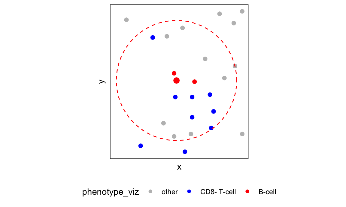
# calculate overall density of cells within each image
# used as "offset" terms in spaMM regression
df_density <- ovarian_df_subset %>%
  group_by(sample_id) %>%
  mutate(n_total = n()) %>%
  group_by(sample_id, phenotype) %>%
  summarise(density = n() / n_total[1]) %>%
  pivot_wider(names_from = phenotype, values_from = density,
                     names_prefix = "density_")
df_nb <- df_nb %>%
  left_join(df_density, by = "sample_id")
spaMM regression
Fit spatial regression using spaMM::fitme. Regression
terms:
vysurvival: the variable of interest.Matern(1|x + y %in% sample_id): Matern spatial correlation term.offset(log(\`density_CD8- T-cell` / (1 - `density_CD8- T-cell`))): offset term for “background” prevalence of CD8- T-cells.
fit_spaMM <-
  fitme(
    formula =
      cbind(`CD8- T-cell`, total - `CD8- T-cell`) ~
      # covariate of interest
      vysurvival +
      # spatial correlation term
      Matern(1|x + y %in% sample_id) +
      # offset term for "background" prevalence of CD8- T-cells
      offset(log(`density_CD8- T-cell` / (1 - `density_CD8- T-cell`))),
    data = df_nb,
    family = binomial(link = "logit"),
    fixed = list("nu" = 0.5),
    method = "ML")
print(fit_spaMM)
## formula: cbind(`CD8- T-cell`, total - `CD8- T-cell`) ~ vysurvival + Matern(1 |
##     x + y %in% sample_id) + offset(log(`density_CD8- T-cell`/(1 -
##     `density_CD8- T-cell`)))
## Estimation of corrPars and lambda by ML (p_v approximation of logL).
## Estimation of fixed effects by ML (p_v approximation of logL).
## Estimation of lambda by 'outer' ML, maximizing logL.
## family: binomial( link = logit )
##  ------------ Fixed effects (beta) ------------
##             Estimate Cond. SE t-value
## (Intercept)    2.303   0.3996   5.764
## vysurvival    -2.002   0.6039  -3.316
##  --------------- Random effects ---------------
## Family: gaussian( link = identity )
##                    --- Correlation parameters:
##       1.nu      1.rho
## 0.50000000 0.01121604
##            --- Variance parameters ('lambda'):
## lambda = var(u) for u ~ Gaussian;
##    x + y %in.  :  1.116
## # of obs: 171; # of groups: x + y %in., 171
##  ------------- Likelihood values  -------------
##                         logLik
## logL       (p_v(h)): -161.5562
Understanding the output of fitme
Many of these are detailed in the documentation
?HLfit.
Fixed effects: estimated coefficients. The conditional standard errors are not very informative, as they do not account for the uncertainty in the random effects term. Below we will perform inferenence on these parameters using likelihood ratio tests instead.
Random effects:
Matern correlation parameters (see
?MaternCorrfor more details):nu: smoothness parameter for the Matern correlation function. We pre-fixed this at 1/2.rho: estimated correlation length for the Matern correlation function. This is the parameter that controls the range of the spatial correlation.Under these specifications, the Matern correlation for two cells with distance
disexp(-rho * d). See?MaternCorrfor more details.
Variance of spatial correlation (
lambda):Details in
?`random-effects`.lambdais the variance of i.i.d normal random variables, which are then multipled by a Cholesky decomposition of the Matern correlation to generate spatially correlated random effects.
LRT testing of fixed effects
We perform LRT on fixed effects by contrasting the fully specified model versus “null” models.
- The intercept is the enrichment of CD8- T-cell colocalizaiton in
B-cell neighborhoods (when
vysurvival = 0), accounting for the “background” chance of CD8- T-cells in the images.
fit_spaMM_null1 <-
  fitme(
    formula =
      cbind(`CD8- T-cell`, total - `CD8- T-cell`) ~
      # null model with no intercept
      0 + vysurvival +
      Matern(1|x + y %in% sample_id) +
      offset(log(`density_CD8- T-cell` / (1 - `density_CD8- T-cell`))),
    data = df_nb,
    family = binomial(link = "logit"),
    fixed = list("nu" = 0.5),
    method = "ML")

1 - pchisq(2 * (logLik(fit_spaMM) - logLik(fit_spaMM_null1)), df = 1)
##         p_v
## 0.002247611- The coefficient for
vysurvivalis whether or not this enrichment is correlated with five-year survival.
fit_spaMM_null2 <-
  fitme(
    formula =
      cbind(`CD8- T-cell`, total - `CD8- T-cell`) ~
      # null model with no vysurvival
      1 +
      Matern(1|x + y %in% sample_id) +
      offset(log(`density_CD8- T-cell` / (1 - `density_CD8- T-cell`))),
    data = df_nb,
    family = binomial(link = "logit"),
    fixed = list("nu" = 0.5),
    method = "ML")

1 - pchisq(2 * (logLik(fit_spaMM) - logLik(fit_spaMM_null2)), df = 1)
##         p_v
## 0.007631282